


Making calculations easier
When we perform calculations in chemistry we are normally concerned with using the most accurate data and exact equations to obtain an acceptable answer. However, there are times when we are justified in making approximations that make calculations easier or even possible at all. In this article I present three examples showing how approximations can be used. I also highlight the importance of ensuring these approximations can be justified.
Equilibrium problems
Much research has been undertaken on the teaching of equilibrium in chemistry.1 Here we will concentrate on one specific mathematical aspect that can make our lives easier while also causing us to consider what is going on beyond the underlying mathematics.
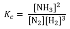
The equilibrium constant Kc for the production of ammonia from hydrogen and nitrogen
N2(g) + 3H2(g) ⇌ 2NH3(g)
is 4.2 x 10⁸ mol-2 dm6 at 298K. From the equation given Kc will be defined as
It follows that for the reverse reaction, the dissociation of ammonia
2NH3(g) ⇌ N2(g) + 3H2(g)
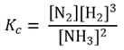
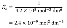
As this is the reciprocal of the expression for Kc for the reverse reaction, for the dissociation of ammonia

| 2NH3(g) | ⇌ | N2(g) | + | 3H2(g) | |
| Initially | 0.25 | 0 | 0 | ||
| Change | −2x | 3x | |||
| At equilibrium | 0.25−2x | 3x |
Let’s now consider what happens when ammonia dissociates. Because Kc is very small there will be much less nitrogen and hydrogen (the products) present in the equilibrium mixture than there are of ammonia (the reactant). Let’s assume that the initial concentration of ammonia is 0.25 mol dm–3, and that in concentration terms 2x of this dissociates to give hydrogen and nitrogen. This table shows the concentrations of the three species present initially and at equilibrium, and the changes that occur.
Note how the quantities are related to the stoichiometry expressed in the reaction equation, which is why the decrease in ammonia concentration was chosen to be 2x.
We can now substitute the concentrations at equilibrium into the expression previously given for Kc.
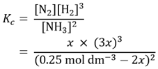
We can, in theory, solve this equation for x since we have the value of Kc. However, this is complicated by the denominator (0.25 mol dm-3 – 2x)2. If we recall the chemistry discussed earlier, we realise the value of x (and consequently of 2x) will be much smaller than 0.25 mol dm−3. If it is sufficiently smaller, we could neglect the −2x term and write an approximate expression for Kc.
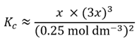
Note the use of the ≈ symbol that denotes an approximation. For now we will assume this is a valid approximation and so we can write
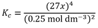
Rearranging this equation to make x4 the subject gives
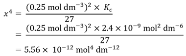
Taking the fourth root of x4 then gives
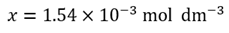
How do we know whether this is a valid approximation? If we attempt to calculate
0.25 mol dm–3 – 2x
We have
(0.25 – 2 x 1.54x10–3) mol dm–3
(0.25 – 3.08x10⁻³) mol dm–3
(0.25 – 0.00308) mol dm–3
Remembering that if we perform a subtraction we are only justified in giving the answer to the same number of decimal places as in the original data, this shows the term being subtracted will be negligible. This is, therefore, a valid approximation.
Real and ideal gases
A very commonly used equation in chemistry is the gas equation
pV = nRT
that relates the pressure p, temperature T and volume V of an amount n of an ideal gas in terms of the gas constant R. Of course, an ideal gas doesn’t actually exist so attempts have been made to modify the equation to more closely predict the behaviour of real gases.
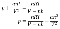
One such modification is the van der Waals equation,2 which is expressed as

This is clearly related to the ideal gas equation, but the pressure has been increased with a term an2/V2, and the volume decreased by nb. The logic behind this is that intermolecular forces reduce the observed pressure so a correction factor needs to be added to give the ideal pressure. This is related to the density of the gas, hence the appearance of n and V. Also, the volume available for the gas molecules to move in is less than that of the container due to the finite size of the molecules themselves. Therefore the volume is reduced by a term which is proportional to the amount n of gas. These terms incorporate constants a and b which are known as the van der Waals constants and are tabulated for different gases.
Let’s consider how both equations predict the behaviour of carbon monoxide gas, for which a = 0.147 Pa m6 mol-2 and b = 3.9 x 10⁻⁵ m3 mol-1. If we rearrange the ideal gas equation we get

At 1000K, if we have 5.0 mol of CO occupying 2.5 m3 then we have
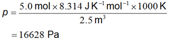
Applying the rules for significant figures and decimal places3 gives a more appropriately expressed result of 17 kPa. Note that in the calculation above I have made use of the relationship 1 Pa = 1 J m-3.
Using the van der Waals equation, successive rearranging gives
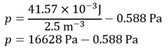
Calculating the values of the various terms in this equation gives
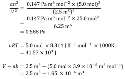
Again, writing this final expression slightly differently gives
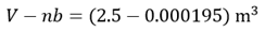
and we see that nb is negligible compared to V.
Putting these together gives
Applying the rules of significant figures3 gives 17 kPa and the an2/V2 term can again be neglected.
Applying the rules of significant figures gives 17 kPa and the an2/V2 term can again be neglected.
It should be apparent that having neglected the -nb and an2/V2 terms reduces the van der Waals equation to the ideal gas equation, so the latter is an appropriate approximation in this case.
It is clear that the approximation to an ideal gas will not be valid when V is small. The term an2/V2 will then be large, and nb is less likely to be negligible relative to V. Real gases are thus likely to deviate from ideal behaviour at high pressures and low temperatures.
Steady state approximation
The steady state approximation doesn’t require us to choose a value for a quantity, but it is still a powerful example of what can be achieved by approximation. It is most commonly used to analyse multi-step reactions.
For example, consider the gas phase decomposition of ozone.
2O3 → 3O2
which is believed to take place via the mechanism
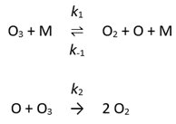
where M can be any molecule.
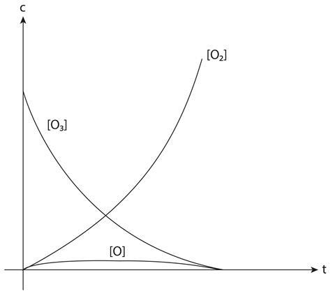
Before analysing this it is helpful to visualise what is taking place using a graph of concentration c against time t. The concentration of O3 falls from its starting value to zero while that of O2 increases from zero at a faster rate. The concentration of the intermediate O increases rapidly from zero but only to a value considerably lower than that of O2 or O3; its value also remains constant for most of the duration of the reaction.
If r1 is the rate at which O2 is produced we can write
r1 = k1[O3][M] + 2k2 [O][O3] – k-1[O2][O][M]
while for the rate r2 at which O3 is produced
r2 = k-1[O2][O][M] – k1[O3][M] – k2[O][O3]
Finally we can write an expression for r3, the rate at which O is produced
r3 = k1[O3][M] – k-1[O2][O][M] – k2[O][O3]
The assumption that we make is that r3 = 0, which is equivalent to assuming that the line representing the concentration of O in the graph is horizontal. This approximation generally works if the concentration of an intermediate is rather lower than that of the products and reactants.
Once we have set
r3 = k1[O3][M] – k-1[O2][O][M] – k2[O][O3] = 0
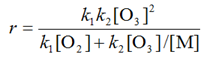
we can perform various algebraic manipulations to show that r, the overall rate for the reaction, is given by
we can perform various algebraic manipulations4 to show that r, the overall rate for the reaction, is given by
The question now arises as to whether the approximation that r3 is zero is reasonable. In this type of example the justification is provided by the extent to which the derived rate equation predicts experimental observations.
Paul Yates is deputy head of academic practice at Newman University
References
- A Raviolo and A Garritz, Chem. Educ. Res. Pract., 2009, 10, 5 (DOI: 10.1039/b901455c)
- J O Valderrama, J. Supercrit. Fluids, 2010, 55, 415 (DOI: 10.1016/j.supflu.2010.10.026)


No comments yet