Using the equation of a straight line

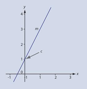
The equation of a straight line is usually taught in the form:

y = mx + c

which succinctly expresses the fact that if we plot y against x and the variables obey a relationship of this form we will obtain a straight line graph with gradient or slope m and intercept (where the line crosses the y-axis) c (fig 1) 

In chemistry the letter c is often used to represent concentration so this is potentially confusing. The letter used to represent the intercept is quite arbitrary, so it is perfectly acceptable to use – as we will for the remainder of this article - the equation in the form y = mx + b as b is a less commonly used symbol. Indeed, this is the form of the equation routinely used in some other countries and several variations are used around the world.

It is important for students to be proficient in using this equation and in understanding the concepts behind it, since many relationships in chemistry can be expressed in linear form. This importance has even led mathematicians to talk of ‘symbol sense’ – an algebraic parallel to the ‘feel for numbers’ known as number sense – that includes the need for everyone to be able to scan a table of data and suggest a symbolic relationship between the variables.¹

Introducing the Equation 

Although the equation of a straight line is well known, it may be worth spending some teaching time exploring it in more detail. It is very straightforward to verify the equation using a specific example, such as:

y = 5x + 2 

It is easy to draw up a table of x against y for a few selected values of x, such as:

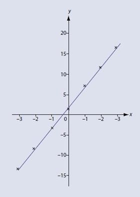
Plotting these data (fig 2) clearly shows that the intercept is 2, while the gradient m can be calculated as:

Of course, more variety can be introduced into this exercise by including decimal values. This also has the advantage of making the results less obvious to those who are already familiar with the concept.

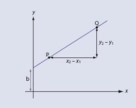
It may be more satisfactory to derive the equation, which again is relatively straightforward. Starting with our definition of the gradient as shown (fig 3):

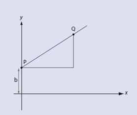
We can move point P so that is located on the y axis (fig 4). A moment’s thought will show that x₁ = 0 and y₁ = b. We then replace x₂ and y₂ with x and y respectively – after all, they are only arbitrary symbols which represent numbers that can vary. The gradient m is now:

We can rearrange this in steps so that:

y– b = mx

and:

y = mx + b

Of course, equations in chemistry are not usually this simple, particularly as the variables are not normally x and y. And it is not just scientists who replace x and y with more complicated symbols and expressions, mathematicians also do this to make the problems more realistic and consequently interesting.²

I usually rewrite the defining equation as:

Y = mX + b

where X is a function of x and Y is a function of y. This is a first step towards moving away from simple x and y variables and accommodates the more complicated functions of variables typically found in equations related to chemistry. It can also be useful to make judicious use of brackets in order to facilitate comparison with equations where the gradient is defined by a combination of constants. A further modification therefore gives:

Y = (m)X + b

Examples from chemistry

1. Beer-Lambert Law

This law is used in spectrometry and states that the absorbance A of a species varies linearly with both the concentration of a solution c and the coefficient of extinction ε, when light passes through a distance known as the path length and denoted by l. The relationship between these quantities is:

A = εcl

If we realise that ε and l will be constant for a specified solution in a cell of fixed path length, we can bracket these constants and write:

A = (εl)c

If we also realise that we can add zero to this without changing the value, we have:

A = (εl)c + 0

Comparing with our defining equation Y = mX + b now gives:

X = c
Y = A
m = εl
b = 0

So plotting A against c will give a straight line graph with gradient εl and intercept of zero. In other words, the graph will go through the origin. 

2. The Nernst Equation

This relates the electromotive force (emf) E of an electrochemical cell to its standard emf E^o and the reaction quotient Q:

where R is the gas constant and F the Faraday constant. Q is calculated from the concentrations of the reacting species while n is the amount of charge transferred in the reaction that occurs. T is the absolute temperature.

First of all we rearrange the equation so that the solitary constant E^o appears at the end:

If we now recognise that T and n will be constants for a given reaction at a specified temperature we can group the constants in the first term in brackets to give:

Comparing with the defining equation Y = mX + b now gives:

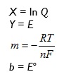
so if we plot E against ln Q we will obtain a straight line and intercept E^o and gradient

3. First order kinetics

Kinetics gives several examples of straight line graphs. Indeed, choosing the appropriate function to plot is a method for determining the order of a reaction. The equation for first order reactions can be written in a number of equivalent forms, which can all be rearranged to give:

ln c = ln c_o– kt

where c_o is the starting concentration of reactant, and c the concentration after time t. The other quantity present is the rate constant k.

The first thing to do when determining what variables to plot is to identify the constants in the equation. The term rate constant gives a strong hint here, and we also need to realise that the starting concentration c_o will be a constant. Further, if c_o is a constant, ln c_o will also be a constant. We move this term to the end of the equation so it becomes:

ln c = -kt + ln c_o

which can be compared to the defining equation Y = mX + b to give:

Y = ln c
X = t
m = -k
b = ln c_o

Consequently, if we plot ln c against t we will obtain a straight line graph with gradient –k and intercept ln c_o.

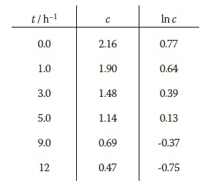
As an example of this, consider the hydrolysis of 1-chloro-1-methylcycloundecane in 80% ethanol at 25^o C.³ We can actually monitor any quantity which is proportional to the concentration, so in this case the values of c are given as relative quantities which do not require units. The table gives the variation of c with time t, along with values of ln c.

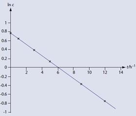
Since this is a first order reaction, the graph of ln c (figure 5) against t is indeed a straight line. The gradient of this graph is -0.13 h^-1. Therefore:

-k = -0.13 h^-1

And:

k = 0.13h^-1

Although this graph and the resulting gradient were generated using spreadsheet software, a study suggested that computing tools may not be as effective as one might expect at developing conceptual understanding in this area.⁴

Paul Yates is the discipline lead in the physical sciences at the Higher Education Academy.

References

- A Arcavi, For the Learning of Mathematics, 1994, 14, 24
- A K Cheng, The Mathematics Educator, 2001, 6, 63
- R J Silbey and R A Alberty, Physical Chemistry. Wiley, 2001
- C Cavanaugh et al, Journal of Educational Computing Research, 2008, 38, 67
No comments yet