Fluorescence lifetime imaging microscopy

Fluorescence lifetime imagingmicrosopy (FLIM) is a non-invasive technique in which an image of a fluorescent probe or marker can be obtained in a cell without compromising or damaging the cell. The combination of scanning laser beams and powerful computers has advanced the field rapidly over the past 20 years. Fluorescence characteristics such as wavelength, lifetime and polarisation can now be recorded relatively easily and quickly. 

Basic principles

Fluorescence is a type of luminescence, ie light generated following the absorption of light (photon) by a suitable molecule (fluorophore). Typically, the molecule is an organic dye, such as fluorescein, which has delocalised electrons. Intrinsic biological molecules, including amino acids such as tryptophan, also fluoresce. 

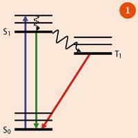
Figure 1 represents a simplified Jablonski energy-level diagram of a fluorophore: the thick black lines represent electronic energy levels; the thin black lines represent vibrational energy levels. On absorption (blue arrow), the molecule moves from its ground electronic state (S₀) to an excited, unstable, electronic state (S₁), which decays back to the ground state either by: 

The emitted luminescence is always at a lower energy (longer wavelength) than the excitation light. This phenomenon was first explained by George Gabriel Stokes in 1852, and the difference in energy between the maxima of the absorption and emission spectra is referred to as the 'Stokes shift' - ie if the molecule is excited with one colour of light, it will emit light of another colour. This is useful because it gives fluorescence microscopy a high contrast - the excitation light can be filtered out and areas without fluorescent molecules are dark.  

In a FLIM experiment, a laser beam is scanned across a sample under a microscope and the fluorescence is measured as a function of the position on the sample. The fluorescence lifetime provides the contrast of the image, which is the basis of fluorescence lifetime imaging.  

The fluorescence lifetime of an isolated fluorophore from a single excited state is given by: 

I(t) =   I₀  e^-t/τf  ( i)   

where (I₀) is the fluorescence intensity at time t  = 0 and (τ_f ) is the fluorescence lifetime (the time after which the fluorescence intensity has decreased by a factor of e ~2.718). 

In the case of a biological sample, the variation in the lifetime of a fluorophore across an image can give valuable information about the biochemical environment. This is because the measured lifetime is dependent on the refractive index of the environment, pH, ion concentration, fluorophore concentration and also on the presence of other molecules which can interact with the excited state by shortening its lifetime (ie quenching of the excited state).^2,3 

Multiple lifetimes may be observed for the cases where there are two or more fluorophores present in the sample or there are different chemical environments experienced by the fluorophore (mixtures of solvents for example). Figure 2 shows the logarithmic fluorescence intensity as a function of time for a single-exponential and a double-exponential decay. (A double-exponential decay is the sum of two single-exponential decays, as in equation (i), but with two different fluorescence lifetimes.)  

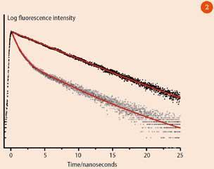
On this scale a single-exponential decay appears linear (filled circles), and the lifetime is calculated as 1/slope of the decay curve (equation (i)). The double exponential (open circles) decay shows two distinct regions.  

Experimental FLIM set-up

A schematic of the FLIM experimental arrangement is shown in Fig 3. A pulsed laser is used to excite the sample, which is mounted on a stage of a laser-scanning confocal microscope. A confocal microscope provides better depth resolution than a standard microscope because it has a pinhole in the beam path which blocks all out-of-focus light.⁴ The fluorescence passes back through the objective lens before it is spectrally separated from the excitation light using a dichroic beam splitter (mirror) and is detected using a photomultiplier tube or photodiode.

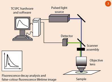
The decay of fluorescence for most biologically important fluorophores typically occurs on timescales on the order of several nanoseconds (1 ns = 10^-9 s). To measure the decay it is therefore essential to use pulses of excitation light which are shorter than the decay time of the fluorophore. Pulsed lasers with picosecond (1 ps = 10^-12 s) or femtosecond (1 fs = 10^-15 s) pulse duration are used. 

The emitted fluorescence photons are detected using time-correlated single photon counting (TCSPC),⁵ which measures the time between the excitation pulse and the arrival of each individual fluorescence photon. A histogram is built up to show the number of fluorescence photons arriving within a given time interval. This curve is fitted to an exponential decay (equation (i)) to obtain the fluorescence lifetime.

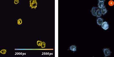
FLIM measures the fluorescence decay in each pixel of an image. Once (τ_f) is obtained for each pixel of the specimen, a FLIM image is created by assigning a false colour scale to the lifetime, eg the shortest detected lifetime is assigned a blue colour and the longest lifetime is assigned red, with a range of colours for intermediate lifetimes.  

An example of a FLIM image is given in Fig 4, showing cells labelled with fluorescent proteins in solutions of different refractive index. The higher the refractive index of the solution, the shorter the fluorescence lifetime, as indicated by the colour in the FLIM image.⁶ 

Fluorescent labels

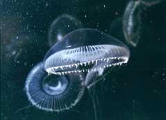
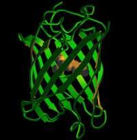
Tagging or labelling a molecule with a fluorescent probe allows us to see exactly where the molecule is located and throws light on its chemical environment. Of particular use in biomedical imaging is the green fluorescent protein (GFP),⁷ which is found in the jellyfish Aequorea victoria. Upon excitation with blue light the GFP fluoresces, emitting green light. Moreover, once fused to a larger protein, GFP can be expressed (created) in vivo.  

In recent years mutants of many different colours have been produced by modifying GFP.^8,9 In 2008 the Nobel prize for chemistry was awarded for the discovery and development of GFP. By labelling different proteins or different parts of the same protein with fluorescent proteins of various colours we can record spectrally-resolved fluorescence images.

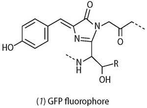
The chemical structure of the GFP fluorophore (1), responsible for the observed fluorescence, is only ca 12Å (1Å= 10^-10 m) in size.⁷ The structure of GFP itself is barrel-like, with the fluorophore located in the centre of 11 β-sheets with a length of around 42Å and diameter of 24Å. The barrel-like structure protects and stabilises the central fluorophore; its small size ensures that the GFP when expressed in vivo does not adversely alter the function of the cell.

Fluorescence imaging of biological samples can be complicated by other molecules inside the cell, such as tryptophan, collagen, elastin, NADH or, in the case of plants, chlorophyll, which also fluoresce.¹⁰ One method of eliminating this 'autofluorescence' from the measured fluorescence intensity is to use a tag or marker with either a spectrally-distinct emission wavelength or a significantly longer fluorescence lifetime than that of the autofluorescence.  

Quantum dots, which are synthesised clusters of semiconducting materials with dimensions of the order of several nanometres (1 nm = 10^-9 m), are one example of a tag currently being used.^11,12 They typically exhibit narrow emission bands, which can be tuned by varying the size of the core of the dot from the ultraviolet (smaller core) to the infrared (larger core), with large absorption cross-sections and long fluorescence lifetimes (up to tens of nanoseconds).  

The photophysical properties of quantum dots, such as quantum yields (brightness) and a reduced susceptibility to fading, appear to be far superior to many organic probes. However, biological applications involving quantum dots have been hindered to an extent by the need to functionalise the surface of the particles so that they become water-soluble and enter the cell. 

Protein interactions

While the resolution of an optical microscope is limited to ca 200 nm, by exploiting Förster Resonance Energy Transfer (FRET),¹³ named after Theodor Förster who explained this effect in the late 1940s, we can identify interactions which occur on significantly shorter length scales. According to Förster, if two fluorescent molecules are <10 nm apart, then a non-radiative transfer of energy is possible between the two.  

For example, if a protein is labelled with one GFP protein (donor) and one red fluorescent protein (RFP) (acceptor), excitation of the GFP may be followed by transfer of its excited state energy to the RFP rather than direct fluorescence emission from the GFP (Fig 5). This is possible only if there is sufficient overlap between the emission spectrum of the GFP and the absorption spectrum of the RFP.

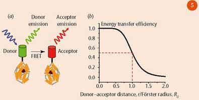
FRET may then be detected by: (i) measuring red fluorescence from the sample; (ii) observing a decrease in the GFP fluorescence intensity; (iii) observing a shorter lifetime component in the GFP decay curve. By photobleaching the acceptor (using light to damage or modify the fluorophore so that it is rendered unable to fluoresce) the FRET pathway can be destroyed and the donor emission lifetime and intensity increase since the molecule can no longer undergo FRET. This effect enables researchers to view interactions between co-localised proteins and infer information about conformational changes and dimerisation in biological systems. As such, FRET has been used in the study of cancer,¹ allergies and immune responses. 

Polarisation resolved anisotropy imaging

Polarisation measurements, which are complementary to lifetime measurements, can yield valuable additional information to FLIM about a sample under study. By exciting a sample using linearly polarised light and measuring the degree of polarisation of the resulting fluorescence, we can determine the rate of tumbling of molecules in a system, which is proportional to the viscosity of the sample.¹⁵ 

There is a finite time period following excitation prior to emission of a photon, and if the molecule has time to tumble in this period then the emission polarisation direction will differ from that of the excitation polarisation. The extent of depolarisation is measured as the fluorescence anisotropy, r, which is related to the rotational correlation time (average tumbling time), Θ, according to the following equation: 

1/r = 1/r₀(1 + τ/Θ)  (ii) 

where r₀ is the initial value of the anisotropy and τ is the fluorescence lifetime.²   

The value of r is the ratio of the difference between the fluorescence intensity recorded parallel and perpendicular to the polarisation of the excitation source to the total fluorescence intensity from the sample. By recording the fluorescence decays parallel and perpendicular to the excitation source for every pixel in a fluorescence lifetime image, it is possible to create time-resolved fluorescence anisotropy images.^14-16 

Contrast in these images can provide evidence for regions of a system with differing viscosity or even reveal the proximity of chemically identical molecules. This is a very exciting technique for cell biology in particular where samples have viscosity gradients and the distribution of protein molecules is of paramount importance for biological function.  

The local viscosity of a cell or compartments within a cell can influence the diffusion of molecules. At higher viscosities, molecules diffuse more slowly, which can lead to slower reaction rates, ie signalling. This has important implications for drug delivery since a higher viscosity may slow down drug delivery. 

Towards a brighter future

Thus FLIM, together with polarisation studies, is proving to be one of the most important and powerful diagnostic tools available for imaging living cells today. 

With new developments in excitation sources and detector technology, FLIM systems with higher resolution and reduced data acquisition times will become available. These advances will allow for real-time in vivo analysis, for example for clinical diagnostics, or for high-throughput screening for drug discovery. 

Looking at the diversity and the potential of the emerging fluorescence techniques, it is clear that the future is bright.

James A. Levitt is a research assistant and Klaus Suhling is a reader in the department of physics at King's College London, Strand, London WC2 2LS; Carolyn Tregidgo is a research scientist at Illumina, Chesterfield Research Park, Essex CB10 1XL.

Acknowledgements

We thank Professor David Phillips and Dr Marina Kuimova in the department of chemistry at Imperial College London, and Nicholas Sergent in the department of physics at King's College London for their helpful comments on this article.

References

- M. Peter et al, Biophysical J., 2005, 88, 1224.
- J. R. Lakowicz, Principles of fluorescence spectroscopy, 3rd edn. New York: Kluwer Academic-Plenum, 2006.
- B. Valeur, Molecular fluorescence. New York: Wiley-VCH, 2002.
- C. J. R. Sheppard, Scanning confocal microscopy. New York: Marcel Dekker, 2003.
- D. V. O'Connor and D. Phillips, Time-correlated single photon counting. New York: Academic,1984.
- C. Tregidgo, J. A. Levitt and K. Suhling, J. Biomed. Optics, 2007, 13, 031218.
- R. Y. Tsien, Ann. Rev. Biochem., 1998, 67, 509
- N. C. Shaner, P. A. Steinbach and R. Y. Tsien, Nature Methods, 2005, 2, 905.
- B. N. G. Giepmanset al, Science, 2006, 312, 217.
- N. Billinton and A. W. Knight, Anal. Biochem., 2001, 291, 175.
- M. G. Green, Angew. Chem. Int. Edn, 2004, 43, 4129.
- D. R. Larsonet al, Science, 2003, 300, 1434.
- T. Förster, Annaleder der Physik, 1948, 6, 55.
- J. Siegel et al, Rev. Scient. Instru., 2003, 74, 182.
- K. Suhlinget al, Optics Lett., 2004, 29, 584.
- A. H. A. Clayton et al, Biophys. J., 2002, 83, 1631.
No comments yet