


Paul Yates looks at extracting information from graphs
In a previous article1 I discussed some of the techniques required in producing graphs, whether drawn by hand or generated using a computer program. I would now like to consider how we extract information from the graph.
One of the most useful quantities we often need to know is the gradient, sometimes referred to as the slope. Frequently its value can be related to a physical quantity that we wish to measure, so it is important to be able to calculate it accurately.
Teaching issues
The images that teachers and students hold of rate have been investigated.2 This study investigated the relationship between ratio and rate, and identified four levels of imagery with increasing levels of sophistication:
- Ratio
- Internalised ratio
- Interiorised ratio
- Rate
The authors describe rate as 'a reflectively-abstracted conception of constant ratio variation'. An investigation of classroom instruction3 found that teaching of this topic was more often done using physical situations than through a functional approach. Problems identified included the recognition of parameters, the interpretation of graphs, and rate of change itself. A more recent study4 looked at the relationship between concepts of gradient, rate of change and steepness, suggesting that textbooks may contribute to misunderstandings of these concepts.
Calculating the gradient
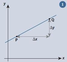
The gradient can be defined using the generic straight line graph (fig 1).
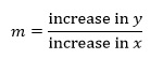
To determine the gradient of the straight line we need to choose two points on the line, here labelled as P and Q. The gradient m of the line between these points is then defined as:
The reason for using the term ‘increase’ for each variable will become apparent shortly.
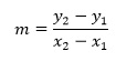
If P has coordinates (x1,y1) and Q the coordinates (x2,y2) we have:
increase in x = x2 – x1
and
increase in y = y2 – y1
so that
we can simplify this slightly using the Greek letter Δ which represents a change in a quantity to give
Where in this case Δx and Δy are interpreted as the increase in x and increase in y respectively. In physical terms, this gradient is called the rate of change of y with respect to x.
In practical terms, the important thing to remember is that more accurate results will be obtained if P and Q are as far apart as possible, as the relative measurement uncertainty is then at its smallest.
Example
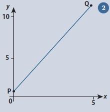
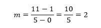
A very simple example (fig 2) will illustrate the technique. P and Q are chosen as two points at either end of the line shown. Their coordinates are (0,1) and (5,11) respectively, so we have

This simple example also serves to provide a simple check that we have the numbers the correct way around. Notice that 11 is directly above 5, both coordinates belonging to point Q. Similarly, the coordinates of P, 1 and 0, appear as y above x.
Examples from chemistry
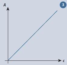
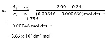
As is often the case, there are new levels of complexity once we start looking at real chemical examples. The Beer-Lambert law
A =εcl
predicts the absorbance A when light passes through a solution of concentration c contained in a cell of path length l, where ε is the molar extinction coefficient. A graph of A against c gives a straight line which passes through the origin (fig 3).
For a solution of bromine in carbon tetrachloride, using an absorption cell with a path length of 1.9 cm and light of 436 nm,5 two points on the line had coordinates:
c1 = 0.000660 mol dm-3, A1 = 0.244
c2 = 0.00546 mol dm-3, A2 = 2.00
So, we have:
Notice how the units have been incorporated into the equation for the gradient as we are dealing with physical quantities, although in this case the absorbance A is a dimensionless quantity and so has no associated units. It is worth remembering that when dealing with real experimental data not all data points will lie on the straight line drawn through them (unless we are fortunate!). The two points used to determine the gradient should, however, lie on the line and do not need to be actual data points.
Negative gradients
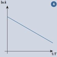
Obtaining the wrong sign on the value of a gradient is a common mistake made by students. There are two ways of dealing with this. One is to recognise that the graph slopes the opposite way (fig 4). The other is to apply the equation for m as given above, ensuring that the coordinates for each pair are positioned one above the other as explained previously. This is why the original definition of gradient above is in terms of an increase in both x and y.
For the reaction:
H2(g) + I2(g)→ 2HI(g)
the rate constant k can be measured as a function of the absolute temperature T. A graph of ln k against 1/T (fig 4) will give a straight line. For this reaction the following points are found to fall on the line:6
The gradient m of the line is then given by:
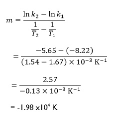
which as expected has a negative value, arising from correct substitution and manipulation of the positive and negative quantities in the equation. This could also have been predicted by recognising that as ln k increases, 1/T decreases. Therefore, in our original definition the increase in 1/T will be negative. Notice also that the logarithmic quantities have no units. Since the gradient is related to the activation energy Ea of the reaction, getting the sign of the value correct is of critical importance.
Curves
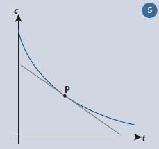
We have seen it is relatively straightforward to determine the gradient of a straight line. It is more complicated with curves. An example is the graph of the reactant concentration c with time for a first order reaction (fig 5). The situation here is that the gradient of the curve is constantly changing. At any point, it is equal to the gradient of the tangent drawn to the curve at that point, such as that shown at P. Since the tangent is a straight line, we can determine the value of its gradient by using the techniques outlined above.
While it is straightforward to determine the gradient of the curve at a specific point, it is clearly impractical if we wish to have a quantitative measure of how the gradient is changing along the curve. Fortunately differential calculus allows us to obtain a general equation for the gradient so we do not need to draw the tangent each time.
Paul Yates is the discipline lead in the physical sciences at the Higher Education Academy and is the author of the book ‘Chemical Calculations’.
Downloads
Complete article
PDF, Size 0.17 mb
References
- P. Yates, Education in Chemistry, 2007, 44, 155
- P.W. Thompson and A.G. Thompson, Annual Meeting of the American
- Educational Research Association, San Francisco, 20-25 April 1992
- S. Stump, Mathematics Education Research Journal, 1999, 11, 124
- D. Teuscher and R.E. Reys, Mathematics Teacher, 2010, 103, 519
- R.J. Silbey and R.A. Alberty, Physical Chemistry, New York, USA: John Wiley & Sons, 2001
- D.D. Ebbing, General Chemistry, , Boston, USA: Houghton Mifflin,1996


No comments yet