In uncertain terms

In this article we return to the proper treatment of data. We have previously seen how to apply descriptive statistics to multiple measurements, and how to ensure that quantities we calculate are expressed to appropriate numbers of significant figures. Here, however, we will discuss how to estimate the likely uncertainty in a single measurement or a small number of measurements.

But first there is an issue of terminology. An overwhelming majority of scientists use the term ‘experimental error’, whereas a minority including myself prefer the term ‘experimental uncertainty’.¹ This is simply because the term ‘error’ implies a mistake, whereas ‘uncertainty’ allows for the fact that no experimental measurements will be exact.

Uncertainty is often introduced in introductory science courses using the concepts of significant figures and by analysing the uncertainty in measurements. It can be a challenging subject to teach,² but studies suggest that the latter method is more likely to result in students understanding what their results mean.

What is uncertainty?

We will begin by considering the simple example of reading a burette. Typically, markings on a burette will be every 0.1 cm³, so it is reasonable to suppose that each reading can be made to ±0.05 cm³. This is the absolute uncertainty and has the same units as the actual reading. We can express a burette reading as

22.85 ± 0.05 cm³

where the ± sign is used to indicate that the value could be higher or lower than that quoted.

We can now calculate the relative uncertainty, which is

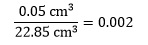
where the units on each quantity cancel. This can be converted to the percentage uncertainty by multiplying by 100, to give 0.2% in this case.

Note that when taking measurements in the laboratory, you should always estimate its uncertainty for use in subsequent calculations.

Maximum possible uncertainty

This is an intuitive approach to uncertainty calculations that provides a useful starting point. Suppose that we have two burette readings from a titration, both with uncertainties

of ±0.05 cm³:

V₁ = 4.65 cm³

V₂ = 21.40 cm³

To determine the titre, we need to calculate V₂ – V₁. A little thought shows that the maximum possible titre will be when V₂ is at its largest and V₁ is at its smallest value. In other words

V₁ = (4.65 – 0.05) cm³ = 4.60 cm³

V₂ = (21.40 + 0.05) cm³ = 21.45 cm³

The titre is then

V₂ – V₁ = (21.45 – 4.60) cm³

= 16.85 cm³

Similarly, the minimum possible titre will be when V₂ is at its smallest and V₁ is at its largest value. This time

V₁ = (4.65 + 0.05) cm³ = 4.70 cm³

V₂ = (21.40 – 0.05) cm³ = 21.35 cm³

The titre is now

V₂ – V₁ = (21.35 – 4.70) cm³ = 16.65 cm³

The difference between the maximum and minimum titres, or the widest possible range of values, is

(16.85 – 16.65) cm³ = 0.20 cm³

We quote the maximum possible uncertainty as plus or minus half this value which is ±0.10 cm³. This assumes that there is equal probability of the uncertainty being positive or negative.

Maximum probable uncertainty

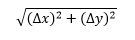
The maximum possible uncertainty is very much a worst case scenario. In most cases the uncertainty will be much smaller. This leads to the concept of the maximum probable uncertainty, which is a little more complicated to calculate but gives more reasonable values. There are two basic rules for combining two quantities x and y with associated uncertainties Δx and Δy.

If x and y are added or subtracted, the overall uncertainty is

For the burette example above, this is

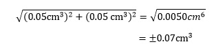
As expected, this is lower than the maximum possible uncertainty of ±0.10 cm³.

If x and y are multiplied or divided, the fractional uncertainty is given by

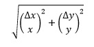
It is important to remember that the fractional uncertainty obtained in this way must be multiplied by the actual value to obtain the absolute uncertainty. The following example shows how this equation can be extended to deal with more than two variables.

An example

A sample of chlorine contains n = 3.5 ± 0.1 mol, at a temperature of 307 ± 2 K and a pressure of 250 ± 5 kPa. Calculate the volume of this sample, together with its associated uncertainty.³

This calculation uses the ideal gas equation which can be rearranged to solve for the volume V:

where R is the gas constant.

Since we are not given R, we need to look it up. An accepted value is 8.314 J K^-1 mol^-1 – but what should we take as the uncertainty in this value? Practically, we can assume that literature values of constants are sufficiently precise that the uncertainty is negligible relative to our calculated values. In fact, it is always worth considering whether any of the uncertainties on measured quantities are so large as to dominate the others or are so small that they can be neglected. This can simplify calculations significantly.

That does not appear to be the case here, so we proceed with the calculation as given. First we need to calculate the value of V, which is given by

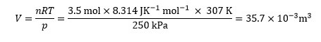
Since the equation contains only multiplication and division, we use the appropriate equation above to determine the fractional uncertainty – in this case with three variables:

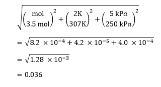
Remembering that this is the fractional uncertainty, we need to multiply it by our value ofV to give the absolute uncertainty as

V = 0.036 x 35.7 dm³

= 1 .3 dm³

The value of the volume is then expressed as

V = 35.7 ± 1.3 dm³

Combining both rules

There are, of course, many calculations that involve combinations of addition, subtraction, multiplication and division. For example, if we wish to calculate the change in standard Gibbs free energy ΔG° for the reaction

HCl_(g) + NH_3(g) → NH₄Cl_(s)

we can use the equation

ΔG° = ΔH° – TΔS°

where ΔH° is the standard enthalpy change and ΔS° is the standard entropy change for the reaction. The absolute temperature is denoted by T. The values for this reaction are:⁴

ΔH° = –176 ± 5 kJ mol^-1

ΔS° = –284 ± 8 J K^-1 mol^-1

T = 298 ± 5 K

We can calculate the TΔS° term in the equation as

298 K × (–284 J K^-1 mol^-1) = –84.6 kJ mol^-1

Since the terms are multiplied, the fractional uncertainty will be

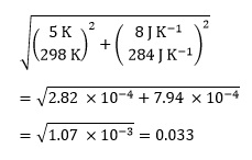
As we are concerned with absolute uncertainties, and each bracket is squared, we do not need to worry about the negative value of ΔS°.

We now multiply the fractional uncertainty by the value of TΔS° to give

0.033 × (–84.6 kJ mol^-1) = –2.8 kJ mol^-1

which is the absolute uncertainty. This is expressed as ±2.8 kJ mol^-1 so again the negative sign is unimportant.

We can now combine the absolute uncertainty on TΔS° with that on ΔH° to give the absolute uncertainty on ΔG° of

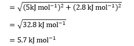
It is straightforward to calculate ΔG° as

ΔG° = –176 kJ – (–84.6 kJ mol^-1)

= –91 kJ mol^-1

So the final value should be expressed as

ΔG° = –91 ± 6 kJ mol^-1

Final notes

It is important to realise that these uncertainty values are only estimates, so it doesn’t make sense to agonise over how many significant figures to include, particularly in intermediate calculations. However, final quantities and their associated uncertainty should be expressed to a consistent number of significant figures. In complicated calculations, try to identify which quantity or quantities will cause most of the uncertainty and concentrate on those.

Paul Yates is the discipline lead for the physical sciences at the Higher Education Academy

This article was updated on 2 July 2014 as the state symbol for NH₄Cl was incorrect. The state symbol for NH₄Cl is now correct.

References

- P Yates, Chemical calculations: mathematics for chemistry, chapter 2. CRC Press, 2007
- R Millar and F Lubben, in G Welford, J Osborne and P Scott (eds) Research in science education in europe, p191–199. Falmer Press, 1996
- D D Ebbing, General chemistry (5th ed.). Houghton Mifflin, 1996S
- S Zumdahl, Chemical principles (3rd ed.). Houghton Mifflin, 1998
No comments yet