Solving equations

Finding solutions to algebraic relationships is a much required skill in chemistry. The common feature of equations is the equals sign, although the precise meaning of this symbol is perhaps not as widely understood as might be presumed. For our purposes, it will be sufficient to realise that if we have an expression containing an equals sign relating a set of variables and constants, we can determine the value of a single unknown quantity by algebraic manipulation. It may be useful to review the previous article on rearranging equations that underpins these techniques.

The equations with which students need to be familiar can essentially be divided into three types: linear equations of a variable; linear equations of a function of a variable; and quadratic equations.

Linear equations of a variable

A very simple example would be

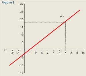
3x – 4 = 17

This is called a linear equation in the variable x due to the power of that variable being 1. If we were to plot a graph of 3x – 4 against x it would be a straight line (fig 1). This equation could be solved graphically by reading off the value of x when the line hits 17 on the vertical scale.

However, it is generally much quicker to solve simple equations like this algebraically. We can add 4 to both sides to give

3x = 17 + 4

∴ 3x = 21

Dividing both sides by 3 then gives

x = 21/3

∴ x = 7

Fortunately, it is very easy to substitute this solution back into the original expression to verify that it is correct.

Linear equations of a function of a variable

An example of this would be

5 lnx + 2 = 10

where lnx is the natural logarithm of the variable x. This is a linear expression in lnx, since a graph of 5 lnx + 2 against x would be a straight line. Solving this equation proceeds as before. We subtract 2 from each side of the equation to give

5 lnx = 10 – 2

∴ 5 lnx = 8

Dividing both sides of the equation by 5 gives

lnx = 8/5

∴ lnx = 1.6

In this case, however, we have one further step – identifying the value ofx that corresponds to lnx = 1.6. To do this we need to use the inverse function of lnx which is the exponential function, e^x. Applying this function to both sides of our equation gives

x = e^1.6

∴ x = 4.95

As before, we can check our solution by substituting this value ofx into the original equation. This will not agree exactly, since the exponential constant, e, is an irrational number, leading to rounding errors. However, the discrepancy is very small.

Quadratic equations

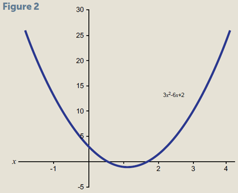
Quadratic equations contain a variable raised to the second power, for example (fig 2):

3x² – 6x + 2 = 0

Not much research has been published on teaching quadratic equations. Most mathematicians would begin by trying to factorise this expression. However, while this approach is fine for simple equations, it is not appropriate for the quadratic equations we will meet in chemistry. It is relatively straightforward to show that for a general equation, expressed in the form

ax² + bx + c = 0

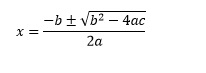
the solutions are given by the equation

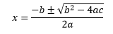
This equation may seem daunting at first, but with some practice it can be memorised. It is sometimes provided as part of lists of equations in examinations. The ± in this equation indicates that we expect two solutions for the quadratic equation. The reason for this may be clearer if we consider a graph.

The function has the value 0 when the curve crosses thex axis. We can see that in the general case this will happen twice. It is also worth noting that b² – 4ac must be positive in order to give real solutions. The situation when it is negative opens up a whole new world of mathematics (imaginary numbers), which certainly has applications in chemistry. However, for now we will simply note that not every quadratic equation has a solution that we can find. Comparing our specific example with the general equation term by term shows that

a = 3, b = –6, c = 2

Then applying the solution equation gives

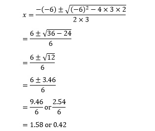
These solutions can again be verified by substituting into the original equation. Because of rounding errors associated with the decimals, this will not give exactly zero. Instead we need to look for a value that is very small with respect to the coefficients in the equation.

Eugenio Filloy and Teresa Rojanao have noted that students take different approaches when moving away from simple types of equation to more complicated ones. There is a spontaneous trial and error phase, before specific strategies are learned to deal with different sets of problems. This is often seen when students move from solving linear to quadratic equations, but is also the basis on which more complicated equations can be solved numerically by computer.

Coming back to chemistry: zero order kinetics

Ammonia decomposing on a platinum surface is a zero order reaction – the rate is independent of the concentration of NH₃. The rate constant¹ k is 2.5 × 10^–4 mol dm^–3 s^–1. For a zero order reaction we can express the concentrationc after time t in terms of the initial concentration c₀.

c = c₀ – kt

If the starting concentration is 0.10 mol dm^–3, we can calculate the time t taken for this to fall to half that value by settingc = 0.05 mol dm^–3 and rearranging to make t the subject. Adding kt to both sides gives:

kt +c = c₀

∴ kt = c₀ – c

Dividing by k gives the expression we need:

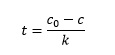
Substituting the known values of c and c₀ into this expression gives

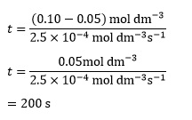
Notice how we use the rules of indices and cancel units to arrive at the final expected units of s.

The Arrhenius equation

This relates the rate constant k for a reaction to the absolute temperature T at which it occurs. In its linear form the equation can be expressed as

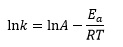
where A is the pre-exponential factor (a constant for a given reaction), E_a is the activation energy and R is the gas constant.

For the substitution reaction between ethyl iodide and hydroxide in ethanol² the activation energy is 90.8 kJ mol^–1. The rate constant k has the value 3.68 x 10^–4 dm³ mol^–1 s^–1 at 305.2 K.

C₂H₅I + OH^–→ C₂H₅OH + I^–

From this data we can calculate the pre-exponential factor A. The first step is to add E_a/RT to both sides of the Arrhenius equation to give

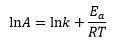
Substituting the values above into this equation:

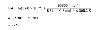
The final step is to undo the effect of the logarithmic function by taking the exponential of this value, so

A = e^27.9 = 1.31 x 10¹²

Degree of dissociation

For chlorine molecules dissociating into atoms

Cl₂→ 2 Cl

if the total volume is 20 dm³, the degree of dissociation α can be found from an equation derived from experimental data³

0.04 α² + (6.86x 10^–3) α– (6.86 x 10^–3) = 0

The decimal coefficients in this quadratic equation are characteristic of such problems in chemistry. Comparing this with the general quadratic equation ax² + bx + c = 0 gives

x =α
a = 0.04
b = 6.86x 10^–3
c = –6.86x 10^–3

Substituting into the general equation

with these values gives us, step by step,

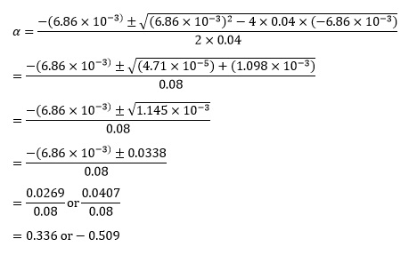
Note that we are subtracting a negative number in the square root, which is equivalent to adding the numbers together.

The ± operator in the equation ensures that we will obtain two solutions, but only one of them is correct. To decide which, we need to think about the chemistry. In this case, the degree of dissociation cannot be negative, so α = 0.336. In other cases the appropriate solution may not be so obvious. As before, we can check our solution by substituting it back into the original equation, but don’t obtain an answer of exactly zero owing to rounding errors. However, once again the discrepancies are small.

Paul Yates is the discipline lead for the physical sciences at the Higher Education Academy.

References

- Class 12 chemistry textbook, chapter 4 (chemical kinetics).
- I N Levine,Physical chemistry. McGraw Hill, 1995
- K J Laidler and J H Meiser, Physical chemistry. Houghton Mifflin, 1999
No comments yet