Journal articles made easy: Detecting iron

This article looks at measuring iron in a variety of solutions using a scalable RGB technique. It will help you understand the research the journal article is based on, and how to read and understand journal articles. The research article was orginally published in Journal of Materials Chemistry A.

Detecting iron the smart way

Solid sensory polymer substrates for the quantification of iron in blood, wine and water by a scalable RGB technique

Click here for full article in Journal of Materials Chemistry A 

Click here for article in Chemistry World

Authors: Saúl Vallejos , Asunción Muñoz , Saturnino Ibeas , Felipe Serna , Félix Clemente García and José Miguel García

Why is this study important?

Iron is present in almost every aspect of our lives but an excess, known as iron overload, can cause significant long term effects ranging from liver damage to arthritis as a result of iron deposition in organs or joints. Because an overdose of iron causes serious problems, it is also an environmental concern. The U.S. Environmental Protection Agency (EPA)¹ and the European Union (EU)² have established limits for iron in drinking water which need to be monitored. Routine blood analysis usually determines the amount of iron in blood serum using ultraviolet-visible spectroscopy (further resources on this technique here and here) to ensure that concentrations are within normal limits. Additionally, cations play an important role in winemaking. The small quantity of iron present in wines is significant as it causes instability; therefore, its concentration must be measured and controlled.

As such, the amount of iron in a variety of environments needs to be carefully monitored.  Current techniques require the use of expensive equipment and must be performed by highly specialised personnel.  In additional, different samples tend to require different processing approaches using current methods.

Further information

• An overview paper on ‘Measurement of environmental pollutants using passive sampling devices’
• Selected further reading from RSC books:
• Carcinogenicity of Metals
• Supramolecular Systems in Biomedical Fields
• The Chemistry of Polymers
• Metal Ions in Toxicology
• The Chemistry and Biology of Winemaking

What is the objective?

The authors aim was to develop a technique to quantitatively measure the amount of iron in a solution which could be completed on-site and at speed. 

What was their overall plan?

• Choose a chemosensor which is capable of detecting Fe(III)
• Introduce a polymerizable chemical group
• Copolymerize with highly hydrophilic co-monomers
• Test that it performs as desired with aqueous samples
• Define the colour change by RGB parameters and use principal componenets analysis to develop a calibration curve
• Anchor the polymer to a film for ease of use
• Cut into circles (sensory discs)
• Test again that it performs as desired
• Test that it performs with the range of substances required (water, blood, wine)
• Ensure that the response time is suitable
• Test selectivity/interference of other cations
• Test whether the desired range of Fe(III) concentrations can be detected

What was their procedure?

Choose a chemosensor which is capable of detecting Fe(III)

To begin, the authors chose one of the best-known chemosensory motifs for detecting Fe(III), 8-hydroxyquinoline (HOx), also known as 8-quinolinol or oxine, because it had been used extensively for the quantitative analysis of a number of metal ions. The mechanism of its chelation is well known.  With iron,   Fe(III)_n:Ox⁻_m complexes are formed with stoichiometries (listed here as n:m) of 1:1, 1:2 and 1:3. The stability constants for these complexes are extremely high, and the structures of the complexes have already been determined by single crystal X-ray crystallography. This, together with the highly coloured nature of the complexes, points to the potential of molecules containing this motif to be used as colorimetric chemodosimeters.  Nevertheless, this organic compound cannot be used as a ferric ion probe for aqueous solutions because it is insoluble in water.

Introduce a polymerizable chemical group

The reaction sequence described below shows how the authors synthesised the methacrylamide monomer HOxMMA which would allow the chemosensor to be polymerised:  

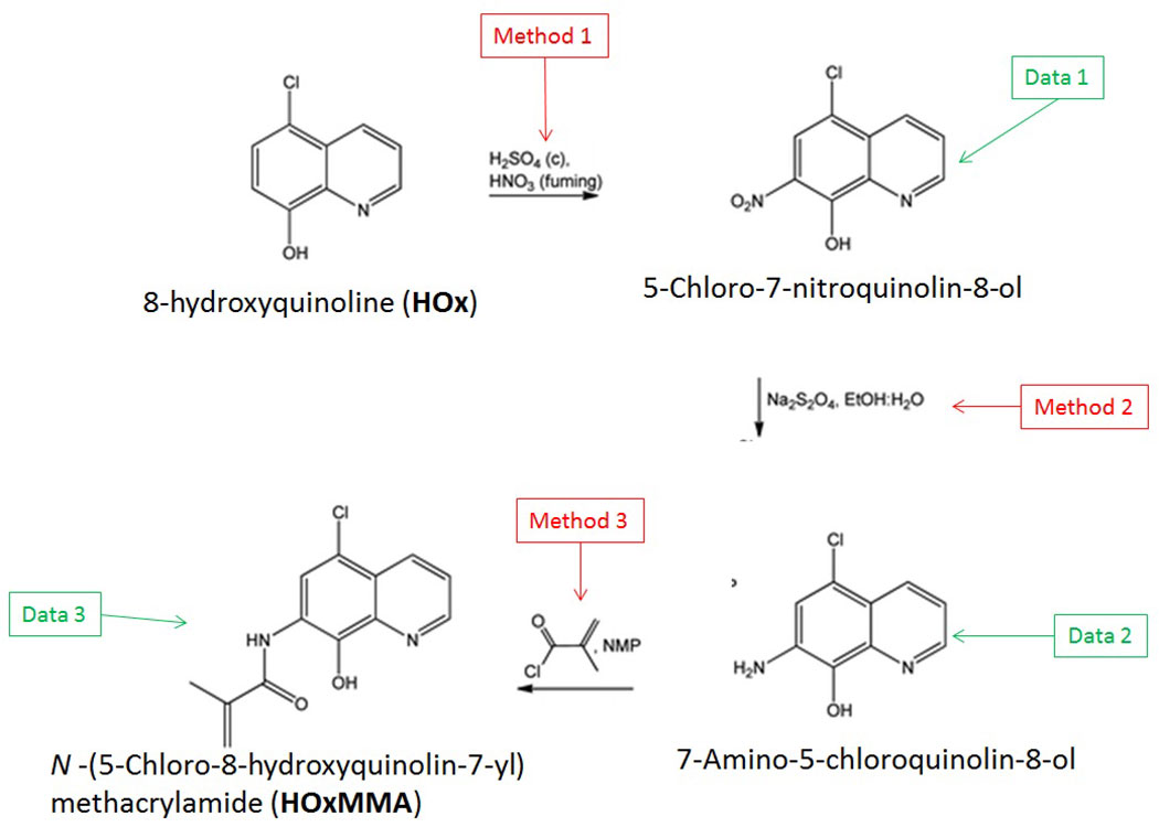
Futher information on the methods used or the data generated in identifying the intermediates, is detailed below:

Method 1

• To a 1 L flask, which was fitted with a mechanical stirrer and a thermometer, was added 111 mmol (20 g) of 5-chloro-8-hydroxyquinoline and 2.24 mol (110 mL) of concentrated sulfuric acid. Afterwards, the system was cooled to 0 °C with an ice bath and 133 mmol (5.7 mL) of fuming nitric acid was added dropwise to the solution, keeping the temperature during the addition lower than 2 °C. The solution was stirred at 0 °C for an additional hour before being warmed to room temperature. It was cautiously poured into ice water, resulting in the precipitation of the product. The heterogeneous system was stirred overnight and the orange solid was filtered off before being washed thoroughly with water and methanol. The product was recrystallized in 2-butanone.
• For information on different practical techniques, illustrating how to assemble the apparatus and with instructional videos click here.
• For animations of the mechanisms for the reaction, click here.

Method 2

• To 100 mL of 50% aqueous ethanol in a round-bottom flask was added 14.96 mmol (3.36 g) of 5-chloro-7-nitroquinolin-8-ol and 78.69 mmol (13.70 g) of sodium dithionite. The mixture was stirred overnight under an atmosphere of nitrogen at room temperature. The yellow solid was filtered off and washed with water. The product was recrystallized in ethanol.
• For information on different practical techniques, illustrating how to assemble the apparatus and with instructional videos click here.
• For animations of the mechanisms for the reaction, click here.

Method 3

• Together with 0.628 g of LiCl, 4.62 mmol (0.9 g) of 7-amino-5-chloroquinolin-8-ol dissolved in 11 mL of NMP was added to a flask equipped with a reflux condenser. Subsequently, 8.31 mmol (0.812 mL) of methacryloyl chloride was added and the solution was stirred for 12 hours at 50 °C under an atmosphere of nitrogen. Finally, the product was precipitated in water. The solid was removed by filtration and treated with water at reflux.
• For information on different practical techniques, illustrating how to assemble the apparatus and with instructional videos click here.
• For animations of the mechanisms for the reaction, click here.

Spectroscopy data

Copolymerize with highly hydrophilic co-monomers

The group then needed to prepare a linear copolymer to link the colorimetric chemosensor with a hydrophilic monomer so that iron concentration in aqueous solutions could be easily measured.  The linear copolymer (LCp) was prepared by radical polymerization of the hydrophilic monomer 2HEA and the sensing monomer HOxMMA in a 99/1 molar ratio, respectively, as shown below.

• A nitrogen gas inlet and a reflux condenser were added to a 100 mL three-necked flask equipped with a magnetic stirrer. Next, 0.4 mmol (105 mg) of HOxMMA and 40 mmol (4.60 g) of 2-hydroxyethyl acrylate (2HEA) were dissolved in DMF (40 mL) and added to the flask. Subsequently, the radical thermal initiator AIBN (656.84 mg, 4 mmol) was added and the solution was heated to 60 °C. After stirring for 4 h under an atmosphere of nitrogen, the solution was allowed to cool before being added dropwise to diethyl ether (300 mL) with vigorous stirring to yield the product as a brown precipitate. The polymer was purified by performing two cycles of the solution/precipitation procedure with methanol (10 mL) as the solvent and diethyl ether (100 mL) as the non-solvent. The final product was dried overnight in a vacuum oven at 60 °C. Yield: 85% (4 g).

Test that it performs as desired with aqueous samples

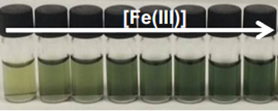
Using the UV/Vis technique (further resources on this technique here and here), an Fe(III) titration with a water solution of LCp was performed. For several samples of different Fe(III) concentration, the authors have recorded the absorbance at differing wavelengths.  Each line on the graph below shows the UV-Vis spectrum for a different concentration of Fe(III).

Upon increasing the Fe(III) concentration, the development of the absorption band at λ_max = 637–651 nm, which corresponds to the formation of complexes with stoichiometries of 1:3 and 1:2, was observed.  The authors have then plotted the absorbance at one particular wavelength (637 nm) against the Fe(III) concentration and produced a titration curve.

Interestingly, the colour development could be followed visually with the deeper the colour development, the higher the Fe(III) concentration.

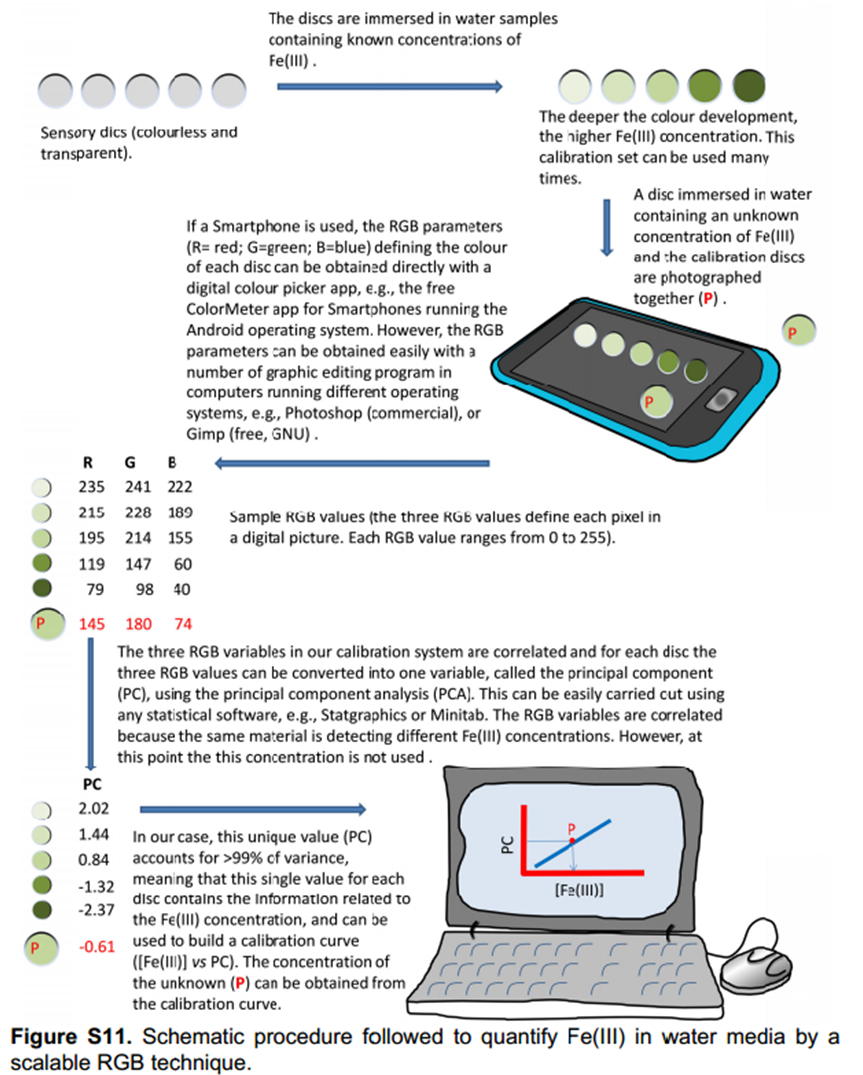
Define the colour change by RGB parameters and use principal componenets analysis to develop a calibration curve

The authors took photos of the different samples on a smartphone and could define each colour by the RGB parameters (R=red; G=green; B=blue).  The RGB values define each pixel in a digital image.   The authors found that the three RGB variables in their calibration system are correlated and so can be converted into one variable, called the principal component (PC), using principal component analysis (PCA).  They could then plot these numbers against Fe(III) concentration to make two titration curves, the first corresponding to a ferric ion concentration maximum of 5.6 ppm and the second corresponding to 560 ppm. The limits of detection and quantification were 493 and 1494 ppb, respectively.  After calculating the titration curves, three test samples that contained 1.7, 3.4 and 18.6 ppm of Fe(III) were measured, providing measured concentrations of 1.8, 3.5 and 17.5 ppm, respectively; these data agreed with the actual ferric ion concentrations and so it was concluded that LCp performs as desired.  

Anchor the polymer to a film for ease of use

At this stage, the authors have developed an effective chemosensor which works in aqueous environments.  However, the aim is to prepare kits for use by non-specialized personnel and so the authors prepared a film Mem, which contained the Fe(III) probe HOxMMA. Mem is a dense membrane with gel-like behaviour in aqueous environments and is manageable when dry or water-swollen. The target molecules enter the membrane, which is where the sensing event takes place, by diffusion into the water-rich membrane gel phase.³

The membrane (Mem) was prepared by the bulk radical polymerization of 1-vinyl-2-pyrrolidone (VP), 2-hydroxyethyl acrylate (2HEA), and N-(5-chloro-8-hydroxyquinolin-7-yl)methacrylamide (HOxMMA) with ethylene glycol dimethacrylate (EGDMMA) as a cross-linking agent and a co-monomer molar ratio VP/2HEA/HOxMMA/EGDMMA of 74/25/1/10. AIBN (1 wt%) was employed as a thermal radical initiator. The bulk radical polymerization reaction was carried out in a silanized glass mould that was 200 μm thick in an oxygen-free atmosphere at 60 °C overnight.

Cut into circles (sensory discs)

The solid sensory substrates were manufactured from Mem films by using a conventional office paper punch to cut out sensory discs that were 5 mm in diameter.

Test again that it performs as desired

The authors then tested these sensory discs to ensure that they performed as required, using the same procedure as previously.  This is outlined in the diagram below.  A reference disc had to be included to determine the ambient light levels so that photos of samples taken in different conditions can be analysed. 

Test that it performs with the range of substances required (water, blood, wine)

The colourless discs were immersed in water that contained between 56 ppb and 56 ppm of Fe(III), white wines that contained between 1.0 and 2.3 ppm of Fe(III), and human blood serum that contained between 1.1 and 10.6 ppm of Fe(III). The disks turned green-brown when exposed to Fe(III) in all environments.  Digital photographs of the discs were used to quantify the Fe(III) content in situ.⁴ After photographing the discs, the three RGB parameters of each disc were processed using principal component analysis as before; the three RGB values of each colour were reduced to one variable (principal component, PC), which permitted the elaboration of the titration curves.

Fig. 2 Titration of Fe(III) using the RGB parameters from digital photographs of the sensory discs immersed in: (a) water, pH = 2, concentration of ferric ions from 56 ppb to 56 ppm; (b) white wine, untreated samples with ferric ion content from 1.0 to 3.4 ppm; and (c) blood serum, untreated samples, from 1.1 to 10.6 ppm. 

Ensure that the response time is suitable

The authors now know that their sensory discs can quantitatively analyse the Fe(III) content in the desired range of aqueous solutions.  However, for this to be useful, the time taken to achieve a result needs to be manageable.  The sensory discs showed a rapid response time of 15 to 30 min for the low ppm range of Fe(III) concentrations. These values were measured with a UV/Vis technique and correspond to the time needed to achieve 90 and 98%, absorbance, respectively (a 99.9% response was obtained after soaking the disk for 60 min).

Test selectivity/interference of other cations

The 8-hydroxyquinoline sub-structure is an effective complexing agent for a number of metal ions and so it was important that the authors test whether the product they had developed was specific to iron or was recording the presence of other cations.  They tested a range of cations [Li(I), Na(I), K(I), Rb(I), Cs(I), Ag(I), Mg(II), Sr(II), Ba(II), Mn(II), Co(II), Ni(II), Cu(II), Zn(II), Pb(II), Cd(II), Hg(II), Cr(III), Zr(III), La(III), Ce(III), Nd(III), Sm(III), Dy(III), Al(III), Cr(VI)] and found that these did not give rise to colour development for water solutions of both LCp and sensory discs.

Fig. 3  UV/Vis response of Mem in water (pH = 2) containing: (a) only Fe(III) and (b) a cocktail of cations: Fe(III), Zn(II), Ni(II), Cu(II), and Mn(II)

Test whether the desired range of Fe(III) concentrations can be detected

In water, a broad range of concentrations were measured, 56 ppb to 56 ppm, covering the EPA and the EU water recommendation ranges for the Fe(III) content in drinking water.

Examination of actual wine samples gave an iron concentration range of 1.0 to 3.4 ppm, thus showing the analytic potential of the sensory material.

In blood serum, the concentration of ferric ions ranged from 1 to 10 ppm, covering the normal range of iron in the blood serum of men, which is 0.8–1.8 ppm.

What are the conclusions?

The authors have prepared colorimetric sensory solid polymer substrates, shaped as discs that are 5 mm in diameter and 0.1 mm in thickness, for the naked-eye detection of iron ions in aqueous environments of special interest in medical, industrial and environmental applications, e.g., in blood serum, wine and drinking water. The colourless and transparent discs turned green-brownish upon immersion in samples containing Fe(III). The colour development was proportional to the concentration of Fe(III), and a simple digital picture of the sensory discs was used to quantify the Fe(III) concentration. The digital definition of the colour of each disc, i.e., the RGB parameters, processed statistically using the principal component analysis (PCA), permitted construction of calibration curves and the measurement of unknowns. Their procedure for quantifying the iron content in beverages, water and biological media in a few minutes by means of a sensory material, a digital camera or a Smartphone, and a computer avoids the usual time-consuming sample preparation, expensive laboratory techniques, and use of specialized personnel required in conventional Fe(III) determination. The chemical composition of the sensory polymer membrane was engineered to give a short response time and to meet special detection requirements (e.g., determining whether the iron content in blood serum is within the normal limits for healthy individuals, or if water and wine have iron concentrations low enough to avoid health or organoleptic problems). Accordingly, the response time of the sensory films was short, 15 min, and the concentrations measured in water ranged from 56 ppb to 56 ppm. This broad range covers the U.S. Environmental Protection Agency EPA and European Union’s (EU) drinking water standards for iron ( %26lt; 300 and 200 ppm, respectively), the typical content of iron in wines (1 to 10 ppm) and the normal range of iron in the blood serum of men (0.8–1.8 ppm).

What are the next steps?

The authors do not talk about their plans to take this work any further.

Could a similar procedure be used to develop techniques for analysing other metal ions in aqueous environments?  What other ions would it be useful to be able to detect in this way?

---

Introduction

For each of the intermediates in the synthesis of HOxMMA, data is provided confirming the identity of the molecules.

For further information on the various spectroscopy techniques used, you can explore our Introduction to spectroscopy tool.  Here you will find an explanation of the principles for a range of spectroscopic techniques including infrared (IR), ultraviolet-visible (UV/Vis) and nuclear magnetic resonance (NMR). Each technique has a drop down box containing clear explanations and descriptions with embedded videos and clickable links to animations (many of which are interactive) to aid your learning.

In addition, our Spectraschool resource gives you the opportunity to look at and compare real spectra of compounds by zooming, overlaying them and pasting them to other documents.  There is also a problem-solving test where your mission will be to identify an unknown compound from an analysis of its spectra - a great tool to check understanding!

¹H-NMR data

The ¹H NMR spectra were recorded with a Varian Inova 400 spectrometer operating at 399.94 MHz for intermediate 1, or on a Varian Mercury 300 spectrometer operating at 299.87 MHz for intermediate 2 and HOxMMA. Deuterated dimethyl sulfoxide (DMSO-d₆) was used as a solvent. 

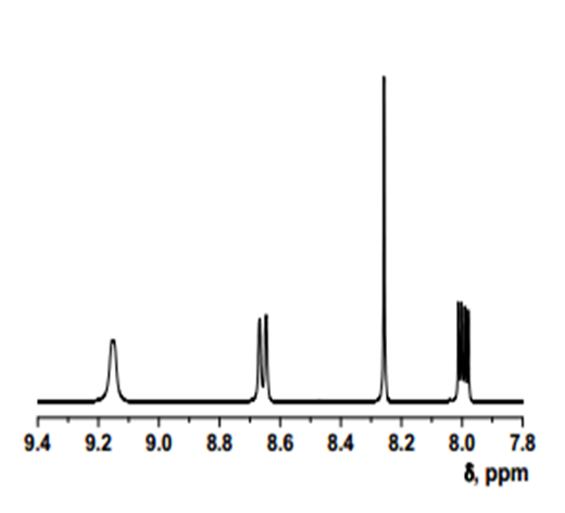
Intermediate 1: 5-Chloro-7-nitroquinolin-8-ol

• 
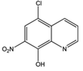
• δ (ppm), 9.15 (d, 1H, 3.9 Hz); 8.67 (d, 1H, 8.4 Hz); 8.26 (s, 1H); 8.01 (dd, 1H, 8.4 and 4.4 Hz).
• 

Intermediate 2: 7-Amino-5-chloroquinolin-8-ol

• 
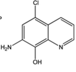
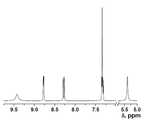
• δ (ppm), 9.42 (s, 1H); 8.78 (d, 1H, 3.9 Hz); 8.29 (d, 1H, 8.4 Hz); 7.35 (m, 1H); 7.34 (s, 1H); 5.36 (s, 2H).
• 

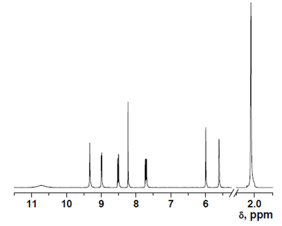
HOxMMA

• 
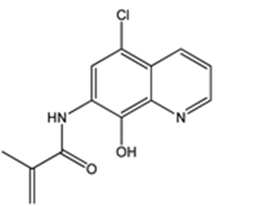
• δ (ppm), 10.72 (s, 1H); 9.32 (s, 1H); 9.00 (d, 1H, 3.9 Hz); 8.53 (d, 1H, 8.4 Hz); 8.23 (s, 1H); 7.73 (dd, 1H, 8.4 and 4.4 Hz); 5.99 (s, 1H); 5.61 (s, 1H); 2.05 (s, 3H). 
• 

¹³C-NMR data

The ¹³C NMR spectra were recorded with a Varian Inova 400 spectrometer operating at 100.58 MHz for intermediate 1, or on a Varian Mercury 300 spectrometer operating at 75.41 MHz for intermediate 2 and HOxMMA. Deuterated dimethyl sulfoxide (DMSO-d₆) was used as a solvent. 

Intermediate 1: 5-Chloro-7-nitroquinolin-8-ol

• 
• δ (ppm), 151.57; 150.98; 141.01; 134.59; 133.23; 129.53; 126.86; 122.99; 118.71. 
• 

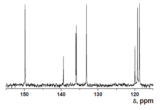
Intermediate 2: 7-Amino-5-chloroquinolin-8-ol

• 
• δ (ppm), 149.82; 139.39; 136.02; 135.879; 133.13; 119.96; 119.24; 118.74; 118.695.
• 

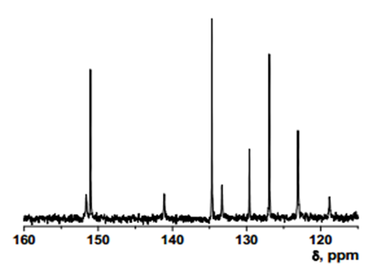
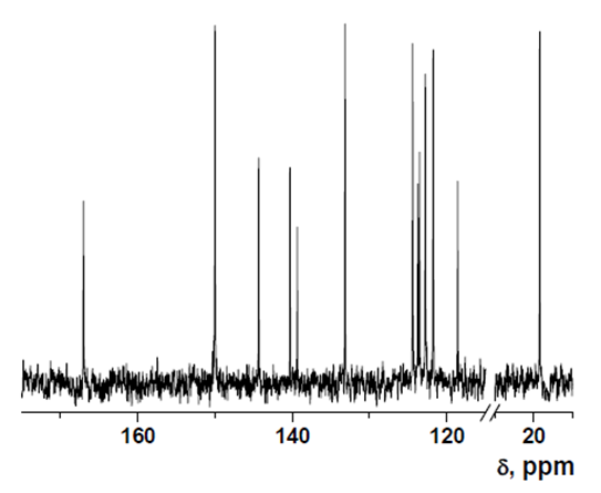
HOxMMA

• 
• δ (ppm), 167.30; 150.27; 144.60; 140.56; 139.62; 133.42; 124.66; 123.99; 123.78; 123.03; 122.02; 118.85; 19.48. 
• 

Further information on NMR spectroscopy:

Vignettes on NMR theory

Exerpt from the book ‘Modern Chemical Techniques’

EI-HRMS data

High-resolution electron-impact mass spectrometry (EI-HRMS) was carried out on a Micromass AutoSpect Waters mass spectrometer (ionization energy: 70 eV; mass resolving power: >10000).

Intermediate 1: 5-Chloro-7-nitroquinolin-8-ol

• 
• m/z: 224 (M+, 100), 150 (90), 194 (55), 115 (46), 166 (45), 226 (35), 114 (25), 152 (21). 

Intermediate 2: 7-Amino-5-chloroquinolin-8-ol

• 
• m/z: 194 (M⁺, 100), 96 (33), 78 (22), 63 (21), 165 (15), 131 (10), 167 (9), 65 (8). 

HOxMMA

• 
• m/z: 262 (M⁺, 100), 193 (88), 41 (86), 69 (55), 165 (63), 264 (37), 195 (32), 129 (29), 221 (27). 

Further information on mass spectrometry:

Introduction to the theory of mass spectrometry.

Exceprt from the book ‘Modern Chemical Techniques’

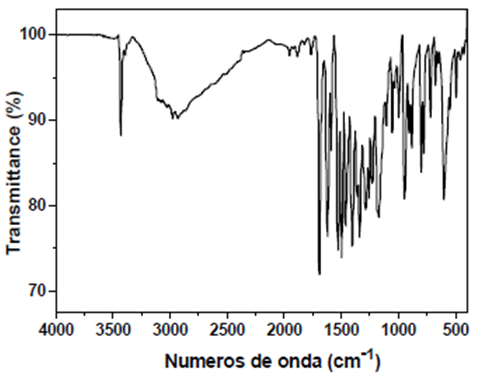
FT-IR data

Infrared spectra (FT-IR) were recorded with a Nicolet Impact spectrometer.

Intermediate 1: 5-Chloro-7-nitroquinolin-8-ol

• 
• FT-IR (wavenumbers, cm⁻¹): ν_O–H: 2808; ν_Ar,CC: 1600; ν_{NO2 (as, s)}: 1503, 1332; ν_C–Cl: 1018.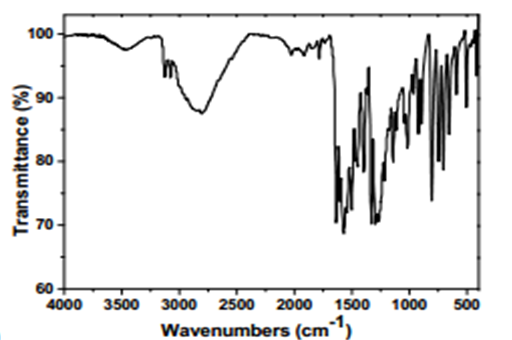 
• 

Intermediate 2: 7-Amino-5-chloroquinolin-8-ol

• 
• FT-IR (wavenumbers, cm⁻¹): ν_C–NH2: 3320; ν_O–H: 3262; ν_Ar,CC: 1588; ν_C–Cl: 1052. 
• 

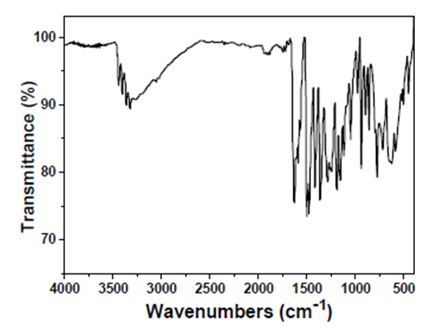
HOxMMA

• 
• FT-IR (wavenumbers, cm⁻¹): ν_N–H: 3441; ν_O–H: 3930; ν_CO: 1692; ν_ArCC: 1585; ν_C–Cl: 1057. 
• 

Further information on infrared spectroscopy:

A video giving instructions on how to run an infrared spectrum.

Short screenshot videos on IR spectroscopy theory.

Introduction to the theory of IR spectroscopy.

---

Dr José M. García, the lead author of the article, answers some additional questions on his group’s work.

What inspired the use of the RGB values as a quantitative technique?

The main goal of our research is to prepare materials by design, i.e. with some properties or characteristics in mind, preparing a material to achieve these technological demands. Regarding this work, our main aim was preparing a material for the visual detection and broad quantification of iron. Our eyes are precise for detecting colours and are obviously valid for analytical purposes. We can detect a colour change and, with a reference, broadly estimate concentrations, for example think of a pH litmus paper, or in  a yes/no pregnacy test. Once a broad estimate is made, our second goal was the use of a conventional device to quantify finely the concentration of the chemical. A conventional digital picture has the colour information taken from a sensory disk, and the RGB parameters can be used to build a calibration curve. If you use a smartphone, the RGB parameters can be directly obtained from the phone. Rapid, cheap, and easy to use from non skilled personnel.

How flexible do you see this technique being for other metals/analytes?

We are working on detecting different chemicals: anions, cations, and neutral molecules. For instance, we are now preparing a paper for visually detecting explosives for civil security purposes. Please see our recent paper in Anal Methods.

In your own words, what do you feel is the highlight of this work?

The design of the sensory material- this is the key to the performance. It is solid, it is sensitive to Fe(III) and can be managed without care, etc.

What do you feel was the biggest challenge in the study?

It is again the capability of preparing materials “a la carte” to achieve technological demands.

How would you like to develop this research in the future?

We have in mind important target molecules to detect for use in civil security, food security and medical fields. Think, for instance, of its use in intelligent fibres that in a garment change colour if a chemical, an explosive, for instance, is in the atmosphere, or intelligent labels for detecting the freshness or the contamination of foods, to name but a few.

How stable are the polymer disks? Do you foresee any issues with storage or usage in the field?

Fully stable for long period of time. The materials can be stored under conventional conditions for months or years.

---

Abbreviations used in text

Abbreviation	Name	Role	Links
HOx	8-hydroxyquinoline	Chemosensory motif	ChemSpider
HOxMMA	N-(5-Chloro-8-hydroxyquinolin-7-yl) methacrylamide	Sensing monomer
2HEA	2-hydroxyethyl acrylate	Hydrophilic monomer	ChemSpider
LCp	Linear copolymer (2HEA + HOxMMA in 99/1 molar ratio)	Linear copolymer for initial testing
VP	1-vinyl-2-pyrrolidone		ChemSpider
EGDMMA	ethylene glycol dimethacrylate	Cross-linking agent	ChemSpider
Mem	Membrane (VP/2HEA/HOxMMA/EGDMMA in a ratio of 74/25/1/10)	Membrane

---

References

1.  U.S. Environmental Protection Agency (EPA), 2012 Edition of the Drinking Water Standards and Health Advisories, EPA 822-S-12-001, http://water.epa.gov/action/advisories/drinking/upload/dwstandards2012.pdf, accessed 16 May 2013.

2.  European Union’s (EU) drinking water standards, Council Directive 98/83/EC of 3 November 1998 on the quality of water intended for human consumption, http://eur-lex.europa.eu/LexUriServ/LexUriServ.do?uri=OJ: L:1998:330:0032:0054:EN: PDF, accessed 2 September 2013.

3.  J. M. Garcia, F. C. Garcia, F. Serna and J. L. de la Peña, Polym. Rev., 2011, 51, 341–390 

4. H. El Kaoutit, P. Estevez, F. C. Garcia, F. Serna and J. M. Garcia, Anal. Methods, 2013, 5, 54–58