Shocking revelations 2: neutralisation reactions

In the previous Exhibition chemistry we saw how to optimise concentrations and reactant volumes to generate a close-to-linear relationship between ion concentration and conductivity – this illustrated the ionic equation for neutralisation reactions for 14–16 students. This time we’ll add some more complexity and nuance for an older audience, using a conductometric titration to study the behaviour differences between weak and strong acids during neutralisations. Please do watch the previous video, as well as this one, before attempting this experiment in front of your class.

Kit

• 25 cm³ of 0.1 mol dm^-3 hydrochloric acid
• 25 cm³ of 0.1 mol dm^-3 ethanoic acid
• 100 cm³ of 0.1 mol dm^-3 sodium hydroxide
• Approx 450 cm³ of deionised water
• 500 cm³ beakers
• Magnetic stirrer
• Clamp and stand
• Burette and burette clamp
• Conductivity probe

Preparation

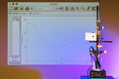
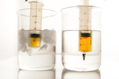
Wear eye protection. Load one of the acids into a beaker and dilute to approx 250 cm³ with deionised water, add a stirrer bead and place on the magnetic stirrer. Use a clamp to position the conductivity probe so that the tip is in the middle of the beaker. Next, position the burette, loaded with the sodium hydroxide solution above the beaker, ensuring the conductivity probe isn’t directly below the jet of the base.

In front of the class

Before starting the experiment, demonstrate the conductivity of the three starting solutions using the probe. The 0.1 M solutions of strong acid and base will both give readings in the tens of thousands of μS/cm, while the weak acid will give well under a tenth of this value. The CLEAPSS conductivity indicator (CLEAPSS members see GL166) clearly displays the difference with the brightness of its LED.

With no precipitation reaction to worry about here, there is no need to be conservative with the burette tap. You can open it fully as soon as your conductivity probe is ready. Once open, log the data collected by the probe for a minimum of around two minutes. Then, repeat the demonstration again with the second acid.

For the neutralisation of the strong (hydrochloric) acid, the conductivity will decrease to a minimum (still above 1000 μS/cm) when half the sodium hydroxide has been delivered. In contrast, the conductivity in the weak (ethanoic) acid titration will increase to the equivalence point – if you’re lucky, you may also see a subtle dip at the beginning before the conductivity rises. After the equivalence point, the conductivity in both titrations will rise at the same rate, as excess sodium and hydroxide ions are added to the mixture.

Teaching goal

This demonstration emphasises the differences in the composition of solutions of strong and weak acids. It would be appropriate at the beginning or end of a unit where comparisons are made between pH curves and conductivity.

Note: the sulfuric(VI) acid used in the previous demonstration had a higher initial conductivity than the hydrochloric acid used in the current experiment. This is due to a higher concentration of hydrogen ions in solution and the additional charge carried by the conjugate base. For the strong acid, the conductivity drops in a near-linear fashion in the initial part of the neutralisation reaction. It then increases from the equivalence point onwards, next the dilution effects become more pronounced and the flow rate from the burette reduces (as the amount of liquid it contains reduces, so does the downwards pressure). 

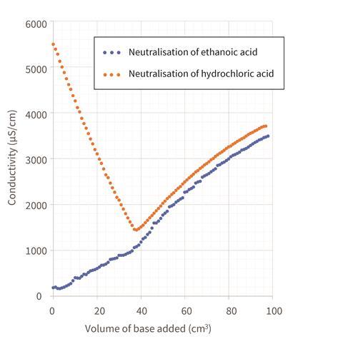
In the previous Exhibition chemistry experiment, we saw the conductivity drop close to zero at the equivalence point as the salt precipitated out of solution, but here the salt remains in solution. However, anyone paying attention ought to wonder why the conductivity drops at all given that the numbers and charges of ions in solution remain constant throughout – with each H⁺ ion being replaced like-for-like with a Na⁺ ion and each Cl^- with a OH^-.

The answer is that hydrogen ions do not exist in solution in isolation (equation 1) but rather as hydronium ions (equation 2).

Equation 1: H⁺ (aq) + OH^- (aq) → H₂ O(l)

Equation 2: H₃ O⁺ (aq) + OH^- (aq) → 2H₂ O(l)

When a potential difference is applied, the Na⁺ and Cl^- ions physically drift through the solution surrounded by a hydration shell of water molecules, which slows them down. By comparison, the hydronium ions, with their exceedingly-labile additional hydrogen need not move at all. Instead they play ‘pass the parcel’ along a chain of neighbouring water molecules to shuffle the charge rapidly through the solution. The hydroxide ions transfer charge in the reverse fashion by stealing hydrogens from their neighbours.

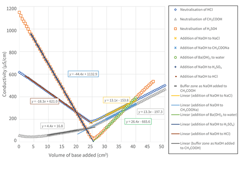
This effect isn’t observed with the weak acid as most of the particles here remain undissociated. Parallels can be drawn between ethanoic acid’s conductometric titration curve and its strong-base pH curve – in which a short, sharp increase in pH occurs before an effective buffer solution is created. This is reflected in the initial subtle dip of the conductivity curve, where the decrease in H₃ O⁺ is not compensated for by the formation of sodium ethanoate. Once the buffer is established, the conductivity increases slowly with the formation of more salt until the equivalence point is reached. From then, the gradient steepens with the addition of the more-highly conductive sodium hydroxide and matches the gradient of the strong acid titration curve after its own equivalence point. As explained in the last issue, the graph begins to curve more noticeably here as the flow from the burette slows and the solution becomes more diluted. The latter effect has been minimised by the addition of water at the start of the demonstration.